Tips on how to Create a Pivot Desk in Excel: A Step-by-Step Tutorial

The pivot desk is one in every of Microsoft Excel’s strongest — and intimidating — capabilities. Pivot tables will help you summarize and make sense of huge knowledge units. Nevertheless, additionally they have a status for being difficult.

The excellent news is that studying tips on how to create a pivot desk in Excel is far simpler than it’s possible you’ll consider.

We’re going to stroll you thru the method of making a pivot desk and present you simply how easy it’s. First, although, let’s take a step again and be sure to perceive precisely what a pivot desk is and why you would possibly want to make use of one.

Desk of Contents

In different phrases, pivot tables extract that means from that seemingly countless jumble of numbers in your display. Extra particularly, it allows you to group your knowledge in several methods so you possibly can draw useful conclusions extra simply.

The “pivot” a part of a pivot desk stems from the truth that you possibly can rotate (or pivot) the information within the desk to view it from a distinct perspective.

To be clear, you’re not including to, subtracting from, or in any other case altering your knowledge once you make a pivot. As an alternative, you’re merely reorganizing the information so you possibly can reveal helpful info.

Video Tutorial: Tips on how to Create Pivot Tables in Excel

We all know pivot tables will be complicated and daunting, particularly if it’s your first time creating one. On this video tutorial, you’ll discover ways to create a pivot desk in six steps and achieve confidence in your capability to make use of this highly effective Excel characteristic.

By immersing your self, you possibly can change into proficient in creating pivot tables in Excel very quickly. Pair it with the beneath package of Excel templates to get began on the precise foot.

What are pivot tables used for?

If you happen to’re nonetheless feeling a bit confused about what pivot tables truly do, don’t fear. That is a kind of applied sciences which might be a lot simpler to grasp when you’ve seen it in motion.

The aim of pivot tables is to supply user-friendly methods to rapidly summarize massive quantities of knowledge. They can be utilized to higher perceive, show, and analyze numerical knowledge intimately.

With this info, you possibly can assist establish and reply unanticipated questions surrounding the information.

Listed here are 5 hypothetical situations the place a pivot desk could possibly be useful.

1. Evaluating Gross sales Totals of Completely different Merchandise

Let’s say you may have a worksheet that comprises month-to-month gross sales knowledge for 3 totally different merchandise — product 1, product 2, and product 3. You need to determine which of the three has been producing essentially the most income.

A method could be to look by means of the worksheet and manually add the corresponding gross sales determine to a working complete each time product 1 seems.

The identical course of can then be performed for product 2 and product 3 till you may have totals for all of them. Piece of cake, proper?

Think about, now, that your month-to-month gross sales worksheet has 1000’s upon 1000’s of rows. Manually sorting by means of every mandatory piece of knowledge may actually take a lifetime.

With pivot tables, you possibly can robotically combination the entire gross sales figures for product 1, product 2, and product 3 — and calculate their respective sums — in lower than a minute.

Picture Supply

2. Displaying Product Gross sales as Percentages of Complete Gross sales

Pivot tables inherently present the totals of every row or column when created. That’s not the one determine you possibly can robotically produce, nevertheless.

Let’s say you entered quarterly gross sales numbers for 3 separate merchandise into an Excel sheet and turned this knowledge right into a pivot desk. The pivot desk robotically provides you three totals on the backside of every column — having added up every product’s quarterly gross sales.

However what in the event you needed to seek out the proportion these product gross sales contributed to all firm gross sales, reasonably than simply these merchandise’ gross sales totals?

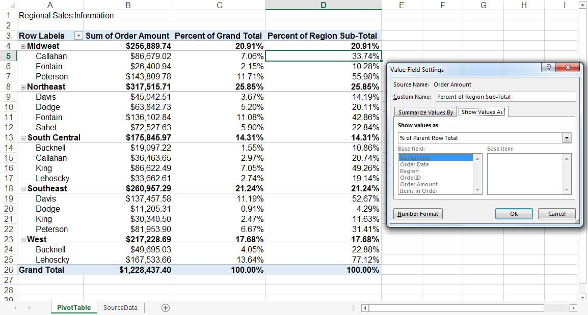
With a pivot desk, as a substitute of simply the column complete, you possibly can configure every column to provide the column’s proportion of all three column totals.

Let’s say three merchandise totaled $200,000 in gross sales, and the primary product made $45,000. You may edit a pivot desk to say this product contributed 22.5% of all firm gross sales.

To point out product gross sales as percentages of complete gross sales in a pivot desk, merely right-click the cell carrying a gross sales complete and choose Present Values As > % of Grand Complete.

Picture Supply

3. Combining Duplicate Knowledge

On this state of affairs, you’ve simply accomplished a weblog redesign and needed to replace many URLs. Sadly, your weblog reporting software program didn’t deal with the change properly and cut up the “view” metrics for single posts between two totally different URLs.

In your spreadsheet, you now have two separate cases of every particular person weblog submit. To get correct knowledge, you have to mix the view totals for every of those duplicates.

Picture Supply

As an alternative of getting to manually seek for and mix all of the metrics from the duplicates, you possibly can summarize your knowledge (by way of pivot desk) by weblog submit title.

Voilà, the view metrics from these duplicate posts shall be aggregated robotically.

Picture Supply

4. Getting an Worker Headcount for Separate Departments

Pivot tables are useful for robotically calculating issues you can’t simply discover in a fundamental Excel desk. A kind of issues is counting rows that every one have one thing in widespread.

As an illustration, let’s say you may have a listing of workers in an Excel sheet. Subsequent to the workers’ names are the respective departments they belong to.

You may create a pivot desk from this knowledge that reveals you every division’s identify and the variety of workers that belong to these departments.

The pivot desk’s automated capabilities successfully eradicate your process of sorting the Excel sheet by division identify and counting every row manually.

5. Including Default Values to Empty Cells

Not each dataset you enter into Excel will populate each cell. If you happen to’re ready for brand new knowledge to return in, you may need a lot of empty cells that look complicated or want additional clarification.

That’s the place pivot tables are available.

Picture Supply

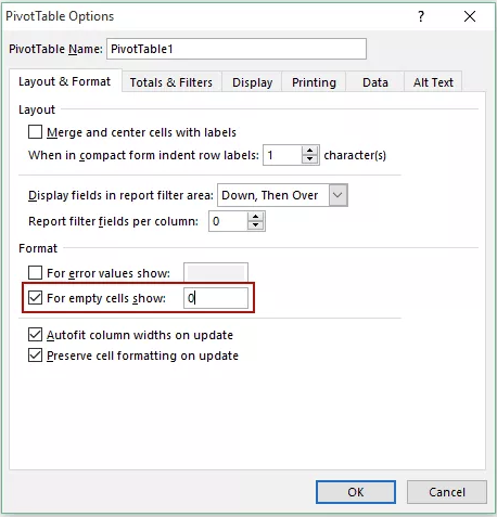
You may simply customise a pivot desk to fill empty cells with a default worth, equivalent to $0 or TBD (for “to be decided”). For big knowledge tables, having the ability to tag these cells rapidly is a beneficial characteristic when many individuals are reviewing the identical sheet.

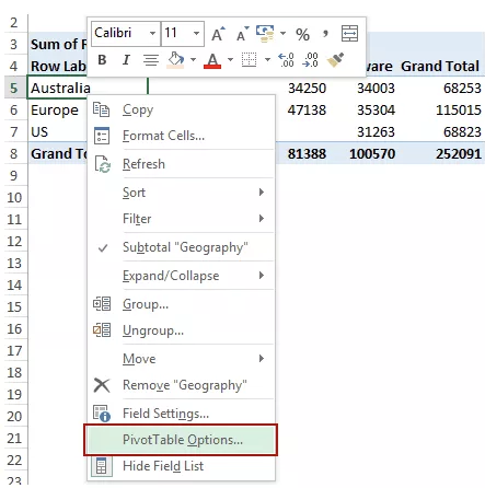
To robotically format the empty cells of your pivot desk, right-click your desk and click on PivotTable Choices.

Within the window that seems, examine the field labeled “For Empty Cells Present” and enter what you’d like displayed when a cell has no different worth.

Picture Supply

Tips on how to Create a Pivot Desk

Now that you’ve got a greater sense of pivot tables, let’s get into the nitty-gritty of tips on how to truly create one.

On making a pivot desk, Toyin Odobo, a Knowledge Analyst, mentioned:

“Apparently, MS Excel additionally offers customers with a ‘Really useful Pivot Desk Operate.’ After analyzing your knowledge, Excel will suggest a number of pivot desk layouts that may be useful to your evaluation, which you’ll be able to choose from and make different modifications if mandatory.

“Nevertheless, this has its limitations in that it might not at all times suggest the most effective association on your knowledge!

“As a knowledge skilled, my recommendation is that you just preserve this in thoughts and discover the choice of studying tips on how to create a pivot desk by yourself from scratch.”

With this nice recommendation in thoughts, listed here are the steps you should utilize to create your very personal pivot desk.

Step 1. Enter your knowledge into a spread of rows and columns.

Each pivot desk in Excel begins with a fundamental Excel desk, the place all of your knowledge is housed. To create this desk, merely enter your values right into a set of rows and columns, like the instance beneath.

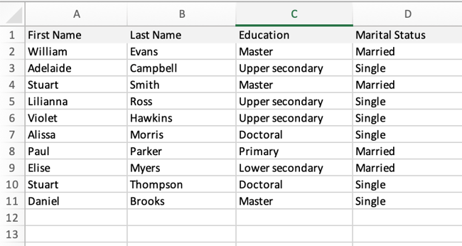
Right here, I’ve a listing of individuals, their training stage, and their marital standing. With a pivot desk, I may discover out a number of items of knowledge. I may learn how many individuals with grasp’s levels are married, as an example.

At this level, you’ll need to have a aim on your pivot desk. What sort of info are you making an attempt to glean by manipulating this knowledge? What would you wish to be taught? It will enable you design your pivot desk within the subsequent few steps.

Step 2. Insert your pivot desk.

Inserting your pivot desk is definitely the simplest half. You’ll need to:

• Spotlight your knowledge.
• Go to Insert within the high menu.
• Click on Pivot desk.

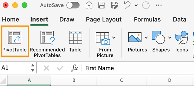
Word: If you happen to’re utilizing an earlier model of Excel, “PivotTables” could also be below Tables or Knowledge alongside the highest navigation, reasonably than “Insert.”

A dialog field will come up, confirming the chosen knowledge set and supplying you with the choice to import knowledge from an exterior supply (ignore this for now). It is going to additionally ask you the place you need to place your pivot desk. I like to recommend utilizing a brand new worksheet.

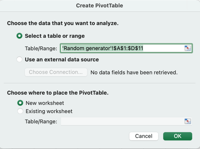
You sometimes received’t must edit the choices except you need to change your chosen desk and alter the situation of your pivot desk.

When you’ve double-checked every thing, click on OK.

You’ll then get an empty consequence like this:

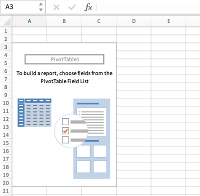
That is the place it will get a bit of complicated, and the place I used to cease as a newbie as a result of I used to be so thrown off. We’ll be modifying the pivot desk fields subsequent so {that a} desk is rendered.

Step 3. Edit your pivot desk fields.

You now have the “skeleton” of your pivot desk, and it’s time to flesh it out. After you click on OK, you will note a pane so that you can edit your pivot desk fields.

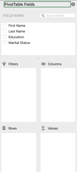
This could be a bit complicated to have a look at if that is your first time.

On this pane, you possibly can take any of your present desk fields (for my instance, it will be First Identify, Final Identify, Training, and Marital Standing), and switch them into one in every of 4 fields:

Filter

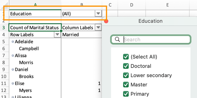
This turns your chosen subject right into a filter on the high, by which you’ll be able to section knowledge. As an illustration, beneath, I’ve chosen to filter my pivot desk by Training. It really works similar to a traditional filter or knowledge splicer.

Column

This turns your chosen subject into vertical columns in your pivot desk. As an illustration, within the instance beneath, I’ve made the columns Marital Standing.

Needless to say the sphere’s values themselves are changed into columns, and never the unique subject title. Right here, the columns are “Married” and “Single.” Fairly nifty, proper?

Row

This turns your chosen subject into horizontal rows in your pivot desk. As an illustration, right here’s what it seems to be like when the Training subject is about to be the rows.

Worth

This turns your chosen subject into the values that populate the desk, supplying you with knowledge to summarize or analyze.

Values will be averaged, summed, counted, and extra. As an illustration, within the beneath instance, the values are a rely of the sphere First Identify, telling me which individuals throughout which academic ranges are both married or single.

Step 4: Analyze your pivot desk.

After you have your pivot desk, it’s time to reply the query you posed for your self firstly. What info have been you making an attempt to be taught by manipulating the information?

With the above instance, I needed to know the way many individuals are married or single throughout academic ranges.

I subsequently made the columns Marital Standing, the rows Training, and the values First Identify (I additionally may’ve used Final Identify).

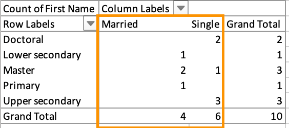
Values will be summed, averaged, or in any other case calculated in the event that they’re numbers, however the First Identify subject is textual content. The desk robotically set it to Rely, which meant it counted the variety of first names matching every class. It resulted within the beneath desk:

Right here, I’ve discovered that throughout doctoral, decrease secondary, grasp, main, and higher secondary academic ranges, these variety of individuals are married or single:

• Doctoral: 2 single
• Decrease secondary: 1 married
• Grasp: 2 married, 1 single
• Major: 1 married
• Higher secondary: 3 single

Now, let’s take a look at an instance of those identical ideas, however for locating the typical variety of impressions per weblog submit on the HubSpot weblog.

Step-by-Step Excel Pivot Desk

1. Enter your knowledge into a spread of rows and columns.
2. Type your knowledge by a selected attribute (if wanted).
3. Spotlight your cells to create your pivot desk.
4. Drag and drop a subject into the “Row Labels” space.
5. Drag and drop a subject into the “Values” space.
6. Tremendous-tune your calculations.

Step 1. I entered my knowledge into a spread of rows and columns.

I need to discover the typical variety of impressions per HubSpot weblog submit. First, I entered my knowledge, which has a number of columns:

• High Pages
• Clicks
• Impressions

The desk additionally consists of CTR and place, however I will not be together with that in my pivot desk fields.

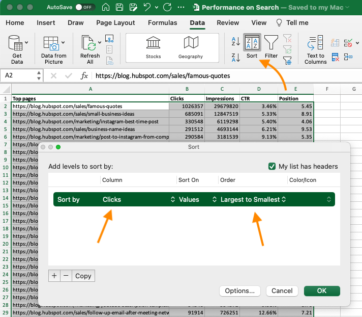
Step 2. I sorted my knowledge by a selected attribute.

I need to kind my URLs by Clicks to make the knowledge simpler to handle as soon as it turns into a pivot desk. This step is elective, however will be useful for big knowledge units.

To kind your knowledge, click on the Knowledge tab within the high navigation bar and choose Type. Within the window that seems, you possibly can kind your knowledge by any column you need and in any order.

For instance, to kind my Excel sheet by “Clicks,” I chosen this column title below Column after which chosen Largest to Smallest because the order.

Step 3. I highlighted my cells to create a pivot desk.

Like within the earlier tutorial, spotlight your knowledge set, click on Insert alongside the highest navigation, and click on PivotTable.

Alternatively, you possibly can spotlight your cells, choose Really useful PivotTables to the precise of the PivotTable icon, and open a pivot desk with pre-set strategies for tips on how to arrange every row and column.

Step 4. I dragged and dropped a subject into the “Rows” space.

Now, it is time to begin constructing my desk.

Rows decide what distinctive identifier the pivot desk will arrange your knowledge by.

Since I need to arrange a bunch of running a blog knowledge by URL, I dragged and dropped the “High pages” subject into the “Rows” space.

Word: Your pivot desk might look totally different relying on which model of Excel you’re working with. Nevertheless, the overall ideas stay the identical.

Step 5. I dragged and dropped a subject into the “Values” space.

Subsequent up, it is time to add in some values by dragging a subject into the Values space.

Whereas my focus is on impressions, I nonetheless need to see clicks. I dragged it into the Values field, and left the calculation on Sum.

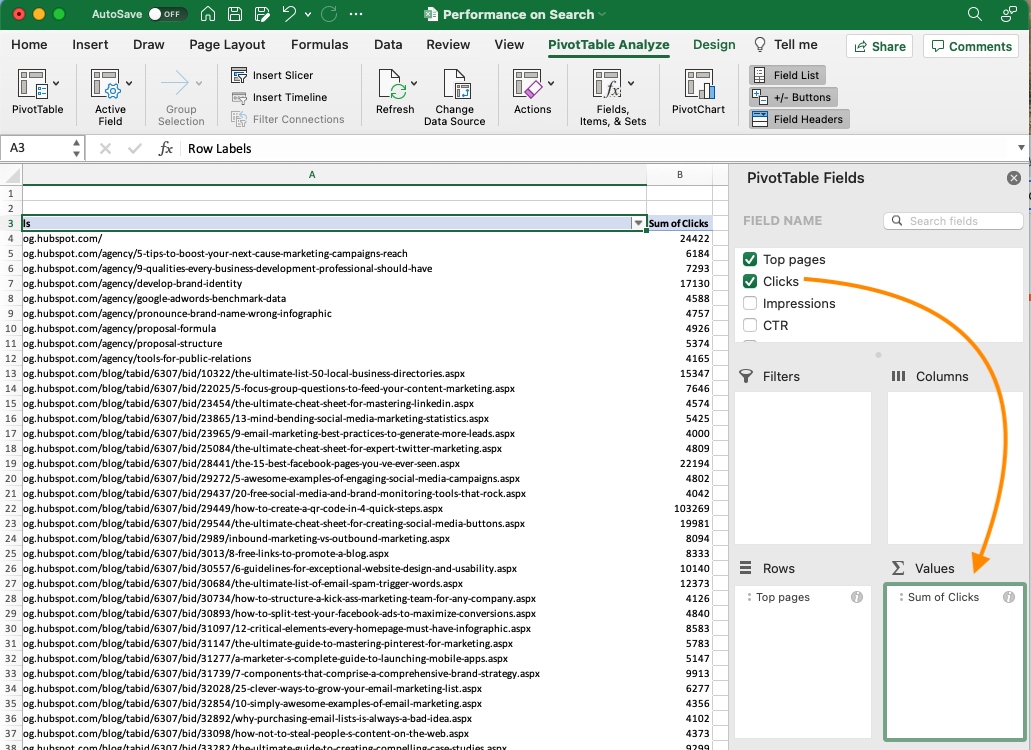
Then, I dragged Impressions into the values field, however I did not need to summarize by Sum. As an alternative, I needed to see the Common.

I clicked the small i subsequent to Impressions, chosen “Common” below Summarize by, then clicked OK.

When you’ve made your choice, your pivot desk shall be up to date accordingly.

Step 6. I fine-tuned my calculations.

The sum of a specific worth shall be calculated by default, however you possibly can simply change this to one thing like common, most, or minimal, relying on what you need to calculate.

I did not must fine-tune my calculations additional, however you at all times can. On a Mac, click on the i subsequent to the worth and select your calculation.

If you happen to’re utilizing a PC, you’ll must click on on the small upside-down triangle subsequent to your worth and choose Worth Subject Settings to entry the menu.

If you’ve categorized your knowledge to your liking, save your work, and do not forget to research the outcomes.

Pivot Desk Examples

From managing cash to conserving tabs in your advertising efforts, pivot tables will help you retain monitor of essential knowledge. The probabilities are countless!

See three pivot desk examples beneath to maintain you impressed.

1. Making a PTO Abstract and Tracker

Picture Supply

If you happen to’re in HR, working a enterprise, or main a small staff, managing workers’ holidays is crucial. This pivot lets you seamlessly monitor this knowledge.

All you have to do is import your workers’ identification knowledge together with the next knowledge:

• Sick time.
• Hours of PTO.
• Firm holidays.
• Time beyond regulation hours.
• Worker’s common variety of hours.

From there, you possibly can kind your pivot desk by any of those classes.

2. Constructing a Funds

Picture Supply

Whether or not you’re working a venture or simply managing your personal cash, pivot tables are a wonderful instrument for monitoring spend.

The best finances simply requires the next classes:

• Date of transaction.
• Withdrawal/bills.
• Deposit/earnings.
• Description.
• Any overarching classes (like paid adverts or contractor charges).

With this info, you possibly can see your greatest bills and brainstorm methods to avoid wasting.

3. Monitoring Your Marketing campaign Efficiency

Picture Supply

Pivot tables will help your staff assess the efficiency of your advertising campaigns.

On this instance, marketing campaign efficiency is cut up by area. You may simply see which nation had the very best conversions throughout totally different campaigns.

This will help you establish ways that carry out properly in every area and the place commercials must be modified.

Pivot Desk Should-Is aware of

There are some duties which might be unavoidable within the creation and utilization of pivot tables. To help you with these duties, we’ve supplied step-by-step directions on tips on how to carry them out.

Tips on how to Create a Pivot Desk With A number of Columns

Now you can create a pivot desk, how about we attempt to create one with a number of columns? Simply observe these steps:

• Choose your knowledge vary. Choose the information you need to embrace in your pivot desk, together with column headers.

• Insert a pivot desk. Go to the Insert tab within the Excel ribbon and click on on the “PivotTable” button.

• Select your knowledge vary. Within the “Create PivotTable” dialog field, be certain that the right vary is robotically chosen, and select the place you need to place the pivot desk (e.g., a brand new worksheet or an present worksheet).

• Designate a number of columns. Within the PivotTable Subject Checklist, drag and drop the fields you need to embrace as column labels to the “Columns” space. These fields shall be displayed as a number of columns in your pivot desk.
• Add row labels and values. Drag and drop the fields you need to summarize or show as row labels to the “Rows” space.

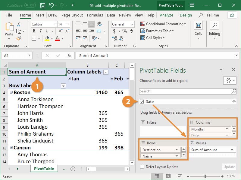
Picture Supply

Equally, drag and drop the fields you need to use for calculations or aggregations to the “Values” space.

• Customise the pivot desk. You may additional customise your pivot desk by adjusting the structure, making use of filters, sorting, and formatting the information as wanted.

For extra visible directions, watch this video:

Tips on how to Copy a Pivot Desk

To repeat a pivot desk in Excel, observe these steps:

• Choose the whole pivot desk. Click on anyplace throughout the pivot desk. You need to see choice handles across the desk.

• Copy the pivot desk. Proper-click and choose “Copy” from the context menu, or use the shortcut Ctrl+C in your keyboard.

• Select the vacation spot. Go to the worksheet the place you need to paste the copied pivot desk.

• Paste the pivot desk. Proper-click on the cell the place you need to paste the pivot desk and choose “Paste” from the context menu, or use the shortcut Ctrl+V in your keyboard.

• Modify the pivot desk vary (if wanted). If the copied pivot desk overlaps with present knowledge, it’s possible you’ll want to regulate the vary to keep away from overwriting the present knowledge. Merely click on and drag the nook handles of the pasted pivot desk to resize it accordingly.

By following these steps, you possibly can simply copy and paste a pivot desk from one location to a different throughout the identical workbook and even throughout totally different workbooks.

This lets you duplicate or transfer pivot tables to totally different worksheets or areas inside your Excel file.

For extra visible directions, watch this video:

Tips on how to Type a Pivot Desk

To kind a pivot desk, you possibly can observe these steps:

• Choose the column or row you need to kind.

• If you wish to kind a column, click on on any cell inside that column within the pivot desk.
• If you wish to kind a row, click on on any cell inside that row within the pivot desk.

• Type in ascending or descending order.

• Proper-click on the chosen column or row and select “Type” from the context menu.
• Within the “Type” submenu, choose both “Type A to Z” (ascending order) or “Type Z to A” (descending order).

Alternatively, you should utilize the kind buttons on the Excel ribbon:

• Go to the PivotTable tab. With the pivot desk chosen, go to the “PivotTable Analyze” or “PivotTable Instruments” tab on the Excel ribbon (relying in your Excel model).

• Type the pivot desk. Within the “Type” group, click on on the “Type Ascending” button (A to Z) or the “Type Descending” button (Z to A).

Picture Supply

These directions will assist you to kind the information inside a column or row in your pivot desk. Please keep in mind that sorting a pivot desk rearranges the information inside that particular subject and doesn’t have an effect on the general construction of the pivot desk.

You can even watch the video beneath for additional directions.

Tips on how to Delete a Pivot Desk

To delete a pivot desk in Excel, you possibly can observe these steps:

• Choose the pivot desk you need to delete. Click on anyplace throughout the pivot desk that you just need to take away.

• Press the “Delete” or “Backspace” key in your keyboard.
• Proper-click on the pivot desk and choose “Delete” from the context menu.
• Go to the “PivotTable Analyze” or “PivotTable Instruments” tab on the Excel ribbon (relying in your Excel model), click on on the “Choices” or “Design” button, after which select “Delete” from the dropdown menu.

Picture Supply

• Verify the deletion. Excel might immediate you to verify the deletion of the pivot desk. Overview the message and choose “OK” or “Sure” to proceed with the deletion.

When you full these steps, the pivot desk and its knowledge shall be faraway from the worksheet. It’s essential to notice that deleting a pivot desk doesn’t delete the unique knowledge supply or some other knowledge within the workbook.

It merely removes the pivot desk visualization from the worksheet.

Tips on how to Group Dates in Pivot Tables

To group dates in a pivot desk in Excel, observe these steps:

• Make sure that your date column is within the correct date format. If not, format the column as a date.

• Choose any cell throughout the date column within the pivot desk.

• Proper-click and select “Group” from the context menu.

Picture Supply

• The Grouping dialog field will seem. Select the grouping choice that fits your wants, equivalent to days, months, quarters, or years. You may choose a number of choices by holding down the Ctrl key whereas making alternatives.

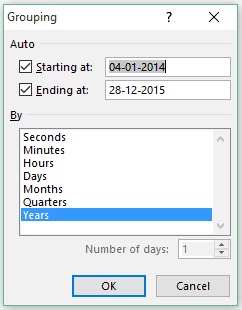
Picture Supply

• Modify the beginning and ending dates if wanted.

• Click on “OK” to use the grouping.

Excel will now group the dates in your pivot desk based mostly on the chosen grouping choice. The pivot desk will show the summarized knowledge based mostly on the grouped dates.

Word: The steps might barely fluctuate relying in your Excel model. If you happen to don’t see the “Group” choice within the context menu, you may as well entry the Grouping dialog field by going to the “PivotTable Analyze” or “PivotTable Instruments” tab on the Excel ribbon, deciding on the “Group Subject” button, and following the following steps.

By grouping dates in your pivot desk, you possibly can simply analyze knowledge by particular time durations, equivalent to months, which will help you get a clearer understanding of developments and patterns in your knowledge.

Tips on how to Add a Calculated Subject in a Pivot Desk

If you happen to’re making an attempt so as to add a calculated subject in a pivot desk in Excel, you possibly can observe these steps:

• Choose any cell throughout the pivot desk.
• Go to the “PivotTable Analyze” or “PivotTable Instruments” tab on the Excel ribbon (relying in your Excel model).
• Go to the “Calculations” group. Within the “Calculations” group, click on on the “Fields, Objects & Units” button and choose “Calculated Subject” from the dropdown menu.
• The “Insert Calculated Subject” dialog field will seem. Enter a reputation on your calculated subject within the “Identify” subject.
• Enter the method on your calculated subject within the “Formulation” subject. You should use mathematical operators (+, -, *, /), capabilities, and references to different fields within the pivot desk.
• Click on “OK” so as to add the calculated subject to the pivot desk.

The pivot desk will now show the calculated subject as a brand new column or row, relying on the structure of your pivot desk.

The calculated subject you created will use the method you specified to calculate values based mostly on the present knowledge within the pivot desk. Fairly cool proper?

Word: The steps might barely fluctuate relying in your Excel model. If you happen to don’t see the “Fields, Objects & Units” button, you possibly can right-click on the pivot desk and choose “Present Subject Checklist.” They each do the identical factor.

Including a calculated subject to your pivot desk helps you carry out distinctive calculations and get new insights from the information in your pivot desk.

It lets you increase your evaluation and carry out calculations particular to your wants. You can even watch the video beneath for some visible directions.

Tips on how to Take away Grand Complete From a Pivot Desk

To take away the grand complete from a pivot desk in Excel, observe these steps:

• Choose any cell throughout the pivot desk.
• Go to the “PivotTable Analyze” or “PivotTable Instruments” tab on the Excel ribbon (relying in your Excel model).
• Click on on the “Subject Settings” or “Choices” button within the “PivotTable Choices” group.
• The “PivotTable Subject Settings” or “PivotTable Choices” dialog field will seem.
• Relying in your Excel model, observe one of many following strategies:
  • For Excel 2013 and earlier variations: Within the “Subtotals & Filters” tab, uncheck the field subsequent to “Grand Complete.”
  • For Excel 2016 and later variations: Within the “Totals & Filters” tab, uncheck the field subsequent to “Present grand totals for rows/columns.”
• Click on “OK” to use the modifications.

The grand complete row or column shall be eliminated out of your pivot desk, and solely the subtotals for particular person rows or columns shall be displayed.

Word: The steps might barely fluctuate relying in your Excel model and the structure of your pivot desk. If you happen to don’t see the “Subject Settings” or “Choices” button within the ribbon, you possibly can right-click on the pivot desk, choose “PivotTable Choices,” and observe the following steps.

By eradicating the grand complete, you possibly can deal with the precise subtotals inside your pivot desk and exclude the general abstract of all the information. This may be helpful once you need to analyze and current the information in a extra detailed method.

For a extra visible clarification, watch the video beneath.

7 Suggestions & Methods For Excel Pivot Tables

1. Use the precise knowledge vary.

Earlier than making a pivot desk, guarantee that your knowledge vary is correctly chosen. Embrace all the required columns and rows, ensuring there aren’t any empty cells throughout the knowledge vary.

2. Format your knowledge.

To keep away from potential points with knowledge interpretation, format your knowledge correctly. Guarantee constant formatting for date fields, numeric values, and textual content fields.

Take away any main or trailing areas, and be certain that all values are within the right knowledge kind.

3. Select your subject names properly.

Whereas making a pivot desk, use clear and descriptive names on your fields. It will make it simpler to grasp and analyze the information throughout the pivot desk.

4. Apply pivot desk filters.

Make the most of the filtering capabilities in pivot tables to deal with particular subsets of knowledge. You may apply filters to particular person fields or use slicers to visually work together along with your pivot desk.

5. Classify your knowledge.

You probably have a considerable amount of knowledge, contemplate grouping it to make the evaluation easier. You may group knowledge by dates, numeric ranges, or along with your particular type of classification.

This helps to summarize and arrange knowledge in a extra significant manner throughout the pivot desk.

6. Customise pivot desk structure.

Excel lets you customise the structure of your pivot desk.

You may drag and drop fields between totally different areas of the pivot desk (e.g., rows, columns, values) to rearrange the structure and current the information in essentially the most helpful manner on your evaluation.

7. Refresh and replace knowledge.

In case your knowledge supply modifications otherwise you add new knowledge, keep in mind to refresh the pivot desk to replicate the newest updates.

To refresh a pivot desk in Excel and replace it with the newest knowledge, observe these steps:

• Choose the pivot desk. Click on anyplace throughout the pivot desk that you just need to refresh.

• Refresh the pivot desk. There are a number of methods to refresh the pivot desk:
  • Proper-click anyplace throughout the pivot desk and choose “Refresh” from the context menu.
  • Or, go to the “PivotTable Analyze” or “PivotTable Instruments” tab on the Excel ribbon (relying in your Excel model) and click on on the “Refresh” button.
  • Or, use the keyboard shortcut: Alt+F5.

• Confirm the up to date knowledge. After refreshing, the pivot desk will replace with the newest knowledge from the supply vary or knowledge connection. We suggest confirming the refreshed knowledge to be sure to have what you need.

By following these steps, you possibly can simply refresh your pivot desk to replicate any modifications within the underlying knowledge. This ensures that your pivot desk at all times shows essentially the most up-to-date info.

You may watch the video beneath for extra detailed directions.

The following tips and tips will enable you create and use pivot tables in Excel, permitting you to research and summarize your knowledge in a dynamic and environment friendly method.

Digging Deeper With Pivot Tables

Think about this. You’re a enterprise analyst. You might have a big dataset that must be analyzed to establish developments and patterns. You and your staff determine to make use of a pivot desk to summarize and analyze the information rapidly and effectively.

As you explored totally different mixtures of fields, you found fascinating insights and correlations that may have been time-consuming to seek out manually.

The pivot desk helped you to streamline the information evaluation course of and current the findings to stakeholders in a transparent and concise method, impressing them along with your staff’s effectivity and skill to retrieve actionable insights. Sounds good proper?

You’ve now discovered the fundamentals of pivot desk creation in Excel. With this understanding, you possibly can determine what you want out of your pivot desk and discover the options you’re searching for. Good luck!

Editor’s word: This submit was initially printed in December 2018 and has been up to date for comprehensiveness.